Tutorial: Hawkes Processes
Here we present an informal introduction to the ideas and theory behind self-exciting (Hawkes) processes. We assume the reader has some familiarity with statistics and machine learning. However, rather than walking the reader through heavy math, we try to highlight the intuition of Hawkes and its potential application areas.
Some Background
Many natural phenomena of interest, to machine learning as well as other disciplines, include time as a central dimension of analysis. A key task, then, is to capture and understand statistical relationships along the timeline. “Workhorse” models addressing temporal data are collected under time-series analysis. Such models often divide time into equal-sized buckets, associate quantities with each such bucket on which the models operate. This is the discrete-time formalism that appears in many models familiar in machine learning such as Kalman filters and hidden Markov models, as well as common models in econometrics and forecasting such as ARIMA or exponential smoothing.
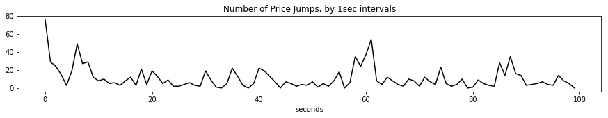
Say we are provided the timestamps of all “price jumps” in a financial market. Exploring this data set from a temporal standpoint, we often take the path of “aggregating” statistics on a uniform time grid, and running models on these aggregates. Concretely, take “millisecond” timestamps of financial market price events:
%matplotlib inline
import numpy as np
import pandas as pd
from matplotlib import pyplot as plt

# here are the "timestamps"
df = pd.read_csv("example_data_top4.csv", header=None)
ar = np.array(df.loc[:, 1])

print ar
[ 56 56 59 ... 8199797 8199798 8199984]
Below, we aggregate them to 1 second intervals –collecting the number of “events” at each interval– to arrive at a familiar “time-series” plot.
# here is the "aggregated" time series plot
bc = np.bincount(np.floor(ar / 1000.).astype(int))

plt.figure(figsize=(15,2))
plt.title("Number of Price Jumps, by 1sec intervals")
plt.xlabel("seconds")
_ = plt.plot(bc[:100], 'k-')
There are many reasons to prefer discrete-time models. First, data may only be collected by a real-world observer (system) in uniform grids of time – and no more granular data is available. Then, of course, more sophisticated models are of little use. Second, these models might be just enough to explain temporal relationships.
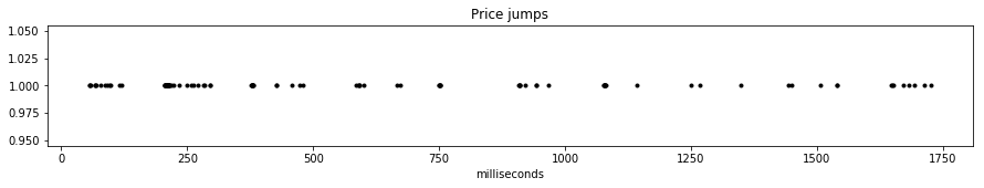
However, many real-world data are available with timestamps. That is, they correspond to discrete events in continuous time. The analyst’s job, then, is to better explain granular temporal relationships, and answer questions like “when is the next event going to occur?”, or “how many events do we expect in the next 5 minutes?”. By basing the analysis on a formalism of continuous time (events can occur at any time) and discrete events (occurrences are instantaneous) , the answers to such questions are unlocked. Furthermore, the framing of the analysis does not depend on arbitrary discretizations of data, that may well lead to loss of valuable information.
Plotting the occurrences themselves, this is more intuitive. Each “point” in the graph is a unique data point, and an arbitrary time “grid” would lead to loss of information.
plt.figure(figsize=(15,2))
plt.title("Price jumps")
plt.xlabel("milliseconds")
_ = plt.plot(ar[:100], np.ones(100), 'k.')
Temporal Point Processes
For dealing with the data above, we will need a few definitions. Stochastic processes are defined as (often infinite) collections of random variables. We will also equip this collection with an index set. For instance, formalizing a model for the “discrete-time” data above, we could write \(\{X_t\}_{t=0}^\infty, t \in \mathbb{Z_+}\). Here \(X_t\) make up the collection while \(\mathbb{Z_+}\) is the index set. The specific dependence (or rather, independence) structure, and other parametric assumptions of relationships among \(\{X_t\}\) determine the stochastic process. Note here that a random variate, or a realization of the process is the entire trajectory determined by values taken by all \(X_t\) (often part of which we observe).
Things are slightly more interesting when the index set is \(\mathbb{R}\). Interpreting the index set as time again, we have arrived at continuous-time processes. Each realization from the process now completely determines a function on domain \(\mathbb{R}\). In machine learning, a Gaussian process is one such example. A staple of quantitative finance, the Wiener process (Brownian motion) is another example.
ar_bm = np.cumsum(np.random.randn(1000) * 0.5**2)
plt.figure(figsize=(15,2))
plt.title("Brownian Motion")
_ = plt.plot(ar_bm, 'g-')
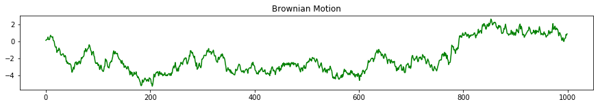
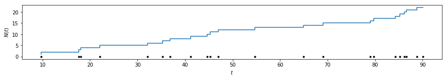
Drawing realizations from both Gaussian and Wiener processes (a stylized example above), we end up with functions \(f: \mathbb{R} \rightarrow \mathbb{R}\). For our purposes, of modeling discrete events, let us restrict this family of possible functions to a special class of step functions defined on \(\mathbb{R}\). Namely, we will deal with functions \(N: \mathbb{R_+} \rightarrow \mathbb{Z_+}\), which are step functions such that \(s > t\) implies \(N(s) \ge N(t)\). We call such processes counting processes.
One possible counting process realization is presented below. Intuitively, the name already suggests one interpretation close to what we are looking for. We can simply take \(N(t)\) to correspond to the “number of occurrences” up to time \(t\). This also suggests that with every counting process, we can associate a probability distribution over points on a timeline. This correspondence is also represented in the figure below. (A technical note here. In making this jump from counting processes to points, we will assume hereforth that no two points coincide, almost surely. In practice, this is rarely an issue.)
This is one way to define temporal point processes, a probability distribution such that each draw is a collection of points on the real line (often the “timeline”). Each “point” will correspond to an “event occurrence” in our example above, and we will use these theoretical devices to explore how “event occurrences” are dispersed throughout time.
ar_pp = sorted(np.random.rand(np.random.poisson(20)) * 100)
f = plt.figure(figsize=(15,2))

plt.step(ar_pp, np.cumsum(np.ones_like(ar_pp)))
plt.ylabel("$N(t)$")
plt.xlabel('$t$')
_ = plt.plot(ar_pp, np.zeros_like(ar_pp), 'k.')
Poisson Process
We start with the simplest temporal point process, the Poisson process. Poisson processes have been described as the simplest process, the process with complete randomness [1], or by Robert Gallager as “the process for which everything we could wish to be true, is true”.
The Poisson process is characterized by complete independence. Other than the point process being simple (no two points coincide), the defining property of Poisson processes is as follows:
The number of occurrences on any two disjoint intervals is independent
The following property is often given in the definition of Poisson processes. Surprisingly, this property is in fact a consequence of the property above (and some other more technical assumptions).
The number of occurrences on an interval \(A\) follows the Poisson distribution,
\[N(A) \sim \mathcal{Po}(\xi(A))\]
Here we have let \(N(A)\) denote the number of points on the interval A, which is itself a random variable of course. \(\mathcal{Po}\) denotes the Poisson distribution. \(\xi\) is a bit more tricky. It is a measure on \(\mathbb{R}\), such that it takes nonnegative values, satisfies \(\xi(\emptyset) = 0\), and the sum of measures of disjoint sets is equal to the measure of the union of such sets. For our purposes, however, let us take
where
We define the function \(\lambda\), the intensity function. For those familiar with probability theory, it should resemble the density function. One way to think about it is that \(\lambda(t)\) defines (in the limit) the probability that there is an occurrence in the infinitesimal interval after time \(t\). So the higher \(\lambda(t)\), the higher the probability of observing points in and around \(t\) (assuming \(\lambda(t)\) is smooth and nice). Let us finally note that the equality above is possible due to our assumption of simplicity – no two points can land on this infinitesimal interval.
Let’s take a step back and recap.
- We define a Poisson process with a function \(\lambda(t) > 0, \forall t\).
- Say we have two intervals, \(A, B \subset \mathbb{R}\). The number of occurrences in these intervals will be Poisson distributed with \(N(A) \sim \int_A \lambda(t)dt\), and \(N(B) \sim \int_B \lambda(t)dt\).
- Most importantly, \(N(A), N(B)\) are independent variables for all \(A \cap B = \emptyset\).
- Higher intensity functions \(\lambda(t)\), as expected, are associated with higher probabilities of event occurrences.
As a concrete example, take the following draws from a Poisson process with \(\lambda(t) = \exp(\sin t))\)
a = np.linspace(0, 100, 10000)
lt = np.exp(np.sin(a))

plt.figure(figsize=(15, 2))
plt.plot(a, lt, 'b-')
plt.yticks([])

for k in range(3):
    count = np.random.poisson(3 * 100)
    smp = [x for x in sorted(np.random.rand(count) * 100) if np.random.rand() * 3 < np.exp(np.sin(x))]
    plt.plot(smp, np.ones_like(smp) * -1 * k, 'k.')
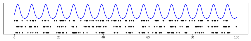
Above, the blue line represents the intensity function \(\lambda(t)\), while each row of black dots is a draw from the Poisson process. Note how the dots have a higher tendency to appear near “peaks” of the intensity function.
That being said, however, the appearance of dots is completely independent. Informally, given \(\lambda(t)\), each event occurs independently and is not affected by whether there are other events in its vicinity.
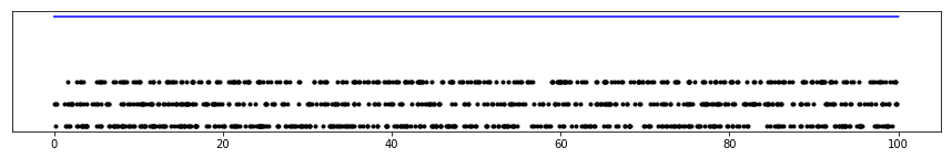
An important special case of the Poisson process is when the intensity function is constant, i.e. \(\lambda(t) = \mu\). We call this special case a homogeneous Poisson process, and it is further characterized by stationarity. Informally, the probability that a point occurs in the vicinity of \(t\) is constant, making it equally likely for points to appear anywhere along the timeline. Concretely, samples from this process would look like (for \(\lambda(t) = 3)\):
a = np.linspace(0, 100, 10000)
lt = np.ones_like(a) * 3

plt.figure(figsize=(15, 2))
plt.plot(a, lt, 'b-')
plt.yticks([])

for k in range(3):
    count = np.random.poisson(3 * 100)
    smp = np.random.rand(count) * 100
    plt.plot(smp, np.ones_like(smp) * -1 * k, 'k.')
We implement homogeneous Poisson processs in
hawkeslib.PoissonProcess.
Poisson processes underlie many applications, for example in queueing theory. There, however, people or packets arriving in a queue can reasonably be expected to obey independence. In many other applications, however, the independence assumption fails basic intuition about the domain. For instance, major financial events are known to draw (excite) others like them. Earthquakes not only occur stochastically themselves, but stochastically trigger others. In these domains, we understand, that Poisson processes lead to an oversimplification. We must work with a more expressive class of models.
Self-exciting Processes
Until now we used the real line on which we defined our point process only rather casually to represent time. The same set \(\mathbb{R}\) can be used to represent distance on a fault line, or depth for example; when carrying out a “cross-sectional” analysis of earthquakes. Here, we will start assigning some meaning to time.
We are looking for ways to break the independence assumption and somehow let event occurrences depend on others. A very natural way to do this is to let the “future” (the rest of the real line deemed not observed) depend on the past. Concretely, on \(\mathbb{R}\), we will let \(\lambda(t)\) depend on the occurrences in \([0, t)\).
In Poisson processes, the intensity function \(\lambda(t)\) was deterministic. Here, let us introduce \(\lambda^*(t)\), the conditional intensity function. \(\lambda^*(t)\) determines the probability of a point occuring in the infinitesimal interval after \(t\), given the events that have occurred until \(t\) (the asterisk will serve as a reminder of this conditioning). In reality, \(\lambda^*(t)\) is a function of \(t\), as well as the occurrences \(\{t_i | t_i < t\}\).
Let’s not get into details here, but it is a fundamental result in the general theory of temporal point processes [1] that we can take \(\lambda^*(t)\), and under a set of mild conditions this will lead to a well-defined point process. Furthermore, such a characterization will enable simplified calculations of likelihood and will be interpretable. See [1] chap. 7 for further details.
Processes defined as above have been called evolutionary, self-modulating, or conditional intensity point processes [1], [2]. In cases where a point occurrence only increases future \(\lambda^*(t)\), another term is more appropriate: self-exciting.
Hawkes Processes
Hawkes processes [3] are often the first and most popular example to evolutionary processes. The (univariate) Hawkes process is defined by the conditional intensity function
Let’s take a minute to break this equation down. At any moment \(t\), the conditional intensity function is at least \(\mu > 0\), the background intensity. However, it also depends linearly on effects of events that have occurred before time \(t\). Namely, this dependence is through a triggering kernel function \(\varphi(.)\), a function of the delay \(t - t_i\) between the current time and the timestamp of the previous event. Note that \(\varphi\) is nonnegative (\(\varphi(x) \ge 0, \forall x \ge 0\) and causal \(\varphi(x) = 0, \forall x < 0\). It is usually a monotonically decreasing function (such as exponential decay, or power-law decay).
Thinking the other way around, the function can be interpreted as follows. Each event that occurs stochastically at a time \(t_i\) adds additional intensity to the process. This added effect often decays throughout time (as governed by \(\varphi\)). In other words, every new occurrence excites the process, hence self-exciting.
The most commonly used kernel function is an exponential decay \(\varphi(x) = \alpha \beta \exp (-\beta x)\). Note that this factorized form, with \(\int \beta \exp (-\beta x) = 1\), leads to a convenient interpretation. \(\alpha > 0\) is known as the infectivity factor, and defines the average number of new occurrences excited by any given occurrence. \(\beta \exp (-\beta x)\), on the other hand is simply the exponential density function that governs the probability distribution of delays between events that excite each other. This is why it is also called the delay density.
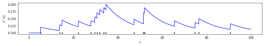
Below is a graphical representation of \(\lambda^*(t)\). Observe how the intensity is stochastically excited by each new arriving occurrence.
from hawkeslib import UnivariateExpHawkesProcess

mu, alpha, beta = .1, .2, .1
uv = UnivariateExpHawkesProcess()
uv.set_params(mu, alpha, beta)
smp = uv.sample(100)

lda_ar = [mu + np.sum(alpha * beta * np.exp(-beta * (x - smp[smp < x]))) \
          for x in np.arange(0, 100, .1)]

plt.figure(figsize=(15,2))
plt.ylabel("$\lambda^*(t)$")
plt.xlabel("$t$")
plt.plot(smp, np.ones_like(smp) * .1, 'k.')
_ = plt.plot(np.arange(0, 100, .1), lda_ar, 'b-')
So far, we discussed “univariate” Hawkes processes. We could assume, however, that each event occurrence bears a discrete mark or label from a finite set. Concretely, going back to our financial example, event occurrences can belong to different types or assets. In this case, one could view the system not only as a single stochastic process, but a finite array of interacting, or mutually-exciting temporal point processes.
Assume observed data is now available as a set of ordered pairs \(\{(t_i, c_i)\}\) where \(t_i \in \mathbb{R_+}\) are the timestamps, and \(c_i \in \{0, 1, \dots, K\}\) are identifiers for which process a given occurrence belongs to. We formalize a multivariate Hawkes process using set of conditional intensity functions
where \(l, k \in \{0, 1, \dots, K\}\) Intuitively, now each process is not only self-excitatory but also excited by events from other processes. Once again, it is common to take a factorized kernel of the form
where now \(A\) is interpreted as the infectivity matrix, and \(A_{l, k}\) is interpretable as the expected number of further type-\(k\) events that will be caused by events of type \(l\).
Likelihood computation, parameter estimation and inference problems in the backdrop of Hawkes processes are not trivial, but they are beyond the scope of this short introduction. See [4], [5] for extensive surveys with a more rigorous treatment of Hawkes processes. Most implementations in this library, and their corresponding API documentation refer to the standard terminology set out in these works.
References
| [1] | (1, 2, 3, 4) Daley, D. J., and D. Vere-Jones. “An Introduction to the Theory of Point Processes: Volume I: Elementary Theory and Methods.” |
| [2] | Cox, David Roxbee, and Valerie Isham. Point processes. Vol. 12. CRC Press, 1980. |
| [3] | Hawkes, Alan G. “Point spectra of some mutually exciting point processes.” Journal of the Royal Statistical Society. Series B (Methodological) (1971): 438-443. |
| [4] | Bacry, Emmanuel, Iacopo Mastromatteo, and Jean-François Muzy. “Hawkes processes in finance.” Market Microstructure and Liquidity 1.01 (2015): 1550005. |
| [5] | Laub, Patrick J., Thomas Taimre, and Philip K. Pollett. “Hawkes processes.” arXiv preprint arXiv:1507.02822 (2015). |