Example: Modeling Seismic Activity
One field where Hawkes processes have traditionally been popular is seismology. In this example, we look at fitting a univariate Hawkes model to earthquakes.
%matplotlib inline
import requests
from lxml import html
from datetime import datetime as dt
import numpy as np
from matplotlib import pyplot as plt
Let’s start by scraping some data on recent earthquakes in and around
Istanbul – where this tutorial was written. The following short script
uses requests, lxml and pandas to scrape some data from the
“recent earthquakes” report maintained by Bogazici University’s
Kandilli Observatory, and whip it
into shape for use.
res = requests.get("http://www.koeri.boun.edu.tr/scripts/lst9.asp")
tx = html.fromstring(res.content).xpath("//pre/text()")[0]
lines = tx.splitlines()[7:]  # get rid of the headers

# take out timestamps and convert them to "hours since first event"
timestamps = [dt.strptime(l[:19], "%Y.%m.%d %H:%M:%S") for l in lines if "ISTANBUL" in l]
t = np.array([(x - ts[-1]).total_seconds() / 3600 for x in timestamps])[::-1]
Estimating Hawkes process parameters
Hawkes processes model self-excitement, systems where point (or event) occurrences excite, or increase the probability of occurrence for, future points. Earthquakes fit this description. Indeed, they are known to trigger after-shocks.
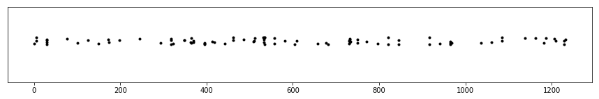
Plotting occurrence times on the timeline, one thing we can expect of aftershock sequences is that they appear “clustered” in time. This is intuitive, a “main” earthquake would occur stochastically (as it would occur in a Poisson process), and the others in the cluster would follow closely after. We plot our data below to verify that this appears to be the case. (We add some “jitter” on the y axis to make viewing easier).
plt.figure(figsize=(15,2))
plt.ylim([-5, 5])
plt.yticks([])
_ = plt.plot(t, np.random.rand(len(t)), 'k.')
We now move to fitting a (univariate) Hawkes process, using the
hawkeslib.UnivariateExpHawkesProcess class. Before we move
on, let’s recap the interpretation of the parameters.
muis the background intensity rate, i.e. the intensity rate for the earthquakes that occur exogenously.alphais the infectivity factor. It can be interpreted as the number of aftershocks, in expectation, to be triggered by each earthquake.thetais the rate parameter of the exponential delay density. For example,thetaequaling to 0.5 would mean that on average 2 hours pass between the main earthquake and the aftershock.
Let’s fit the model.
%%time
from hawkeslib import UnivariateExpHawkesProcess as UVHP

uv = UVHP()
uv.fit(t)
print uv.get_params()
(0.04930555306217892, 0.30548369162341404, 5.150339498582191)
CPU times: user 1.48 ms, sys: 0 ns, total: 1.48 ms
Wall time: 1.44 ms
Interpreting the parameters, we conclude that earthquakes occur
exogenously once every ~20 hours in Istanbul (here, we call any
registered seismic activity an “earthquake”). Each main shock results in
0.3 aftershocks on average, and aftershocks occur with
1 / 5.15 = 0.194 delay or 12 minutes on average.
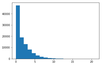
Having fit a model, hawkeslib allows sampling (unconditional) from
the model, as well as evaluate likelihood (e.g. for out-of-sample cross
validation) for other data sets. Here, let’s take a few samples from the
“earthquake timeline” and use it to approximate the histogram for the
number of tremors during a 24 hour time span in the city.
nr_shocks_sample = [len(uv.sample(24)) for x in range(100000)]
_ = plt.hist(nr_shocks_sample, bins=20)
Bayesian inference
Having fit the model, we now move to quantifying uncertainty in the
parameter estimates. In hawkeslib, we do this by Bayesian inference
in the univariate Hawkes model. Related functionality is implemented in
hawkeslib.BayesianUVExpHawkesProcess.
Below, we use hawkeslib to sample from the posterior
distribution of parameters mu, alpha, and theta. We then
present “Bayesian credible intervals” for the parameters.
from hawkeslib import BayesianUVExpHawkesProcess as BUVHP

buv = BUVHP(mu_hyp=(1., 10.), alpha_hyp=(1., 1.), theta_hyp=(1., 10.))
trace = buv.sample_posterior(t, T=t[-1], n_samp=50000)
# compute the BCIs
print pm.stats.quantiles(trace["alpha"], [2.5, 97.5])
print pm.stats.quantiles(trace["theta"], [2.5, 97.5])
{2.5: 0.19881998542628126, 97.5: 0.45850986170997604}
{2.5: 2.9138895786443646, 97.5: 8.605057427283178}
We observe that, under small data the credible intervals around our parameters are relatively wide.
Let us end by noting that a more expressive model, one that takes into account earthquake magnitudes, would be required for more realistic scenarios. Traditionally, this is a marked Hawkes process that’s known as ETAS, the Epidemic-type Aftershock Sequence Model [1].
References
| [1] | Ogata, Yosihiko, Ritsuko S. Matsu’ura, and Koichi Katsura. “Fast likelihood computation of epidemic type aftershock‐sequence model.” Geophysical research letters 20.19 (1993): 2143-2146. |